Week 2 - Revisiting Parisi's Equations and the Replica Method

Recap of the Meeting

We spent most of our time discussing geometric intuition for the dynamics described by the Parisi’s PDEs.

• The equations are given as $$ \begin{cases} \Phi_t(t, x) = - \frac{\beta^2}{2} \cdot \big( \Phi_{xx}(t, x) + \mu(t) \cdot \lvert \Phi_x(t, x) \rvert^2 \big) \\ \Phi(1, x) = \log \big( 2 \cdot \cosh x \big) \end{cases} $$

• When a change of variable is performed $t(s) = 1 - s$, the PDE becomes $$ \begin{cases} \Phi_s(s, x) = \frac{\beta^2}{2} \cdot \big( \Phi_{xx}(s, x) + \mu( 1 - s ) \cdot \lvert \Phi_x(s, x) \rvert^2 \big) \\ \Phi(0, x) = \log \big( 2 \cdot \cosh x \big) \end{cases} $$

• The behavior of this dynamic can be interpreted as follows. At time $s = 0$, we begin with the soft absolute value function $\Phi(0, x) = \log \big( 2 \cdot \cosh x \big)$. As $s$ progresses from $0 \rightarrow 1$, the evolution of $\Phi(s, x)$ is always affected by heat diffusion dynamics $$- \frac{\beta^2}{2} \cdot \Phi_{xx}(t, x)$$

• On the other hand, $\mu(1 - s)$ is non-increasing on the interval $[0, 1]$. The function $\mu(s)$ itself is the cumulative density function of some measure supported on $[0, 1]$. Thus, the evolution of $\Phi(s, x)$ is also affected by a “gradient descent” dynamic $$\frac{\beta^2}{2} \cdot \lvert \Phi_x(s, x) \rvert^2$$ whose weight is dampened as $s$ increases towards $s = 1$.

This picture was helpful to have. It plots the evolution of $\Phi(s, x)$ from $s = 0 \rightarrow 1$

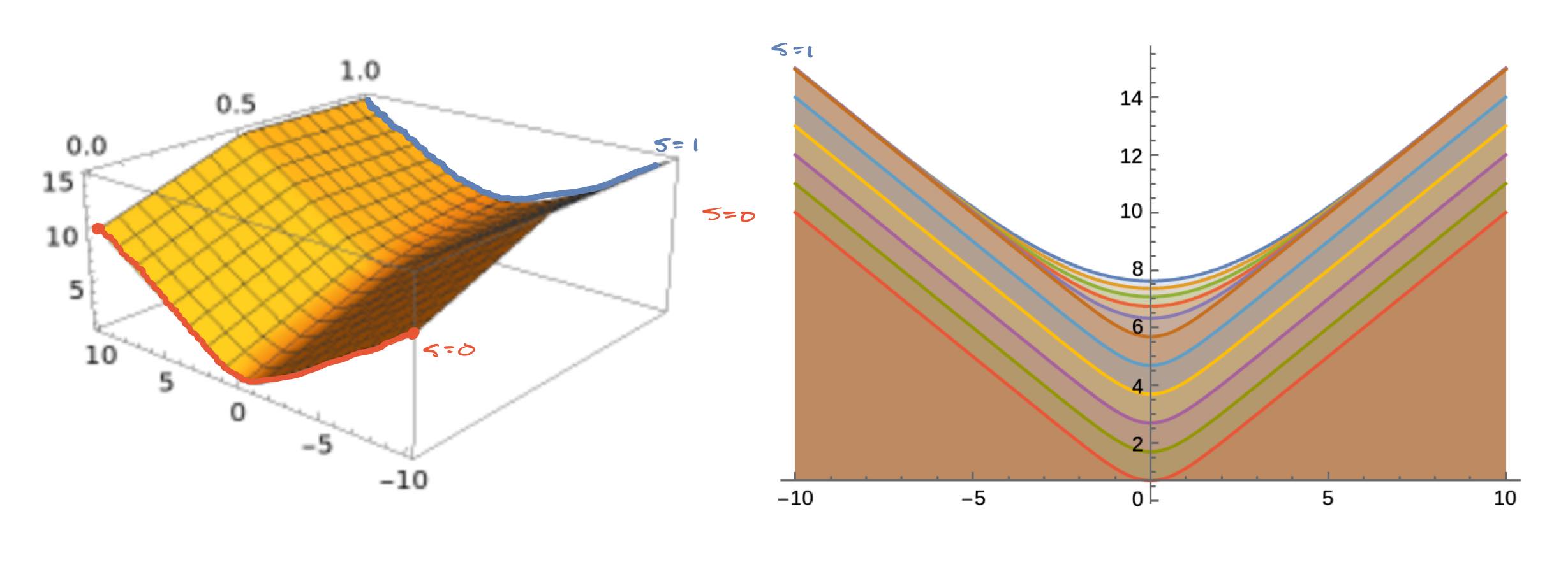
where, on the right, the red contour corresponds to $s = 0$, the navy contour corresponds to $s = 1$, and $\mu(t)$ is given by the CDF of a Gaussian centered at $\frac{1}{2}$ with variance $\frac{1}{100}$

When thinking of $\mu(1 - s)$, consider the above picture as “backwards” i.e. think of $t$ progressing from $1 \rightarrow 0$.

Material

• [pdf] Scanned presentation notes

• [demo] [source] Plotting Parisi’s equations

• [link] Scribe notes – Juspreet Singh Sandhu (see Day 2)